
Machine Learning : Handling Dataset having Multiple Features
In real world scenarios often the data that needs to be analysed has multiple features or higher dimensions. The number of features might be in two or three digits as well. If lots of the features are responsible for statistics then it becomes a complex learning problem to solve for such datasets. This is referred as Multivariate statistics which is a subdivision of statistics encompassing the simultaneous observation and analysis of more than one outcome variable.
Often if dataset is simple enough having two dimensions (X & Y), for instance a set of medicines having only two properties, weight index and pH, based on which dataset to be classified then K-Means clustering technique suits. But that does not work well when there are many different features are involved from which you are trying predict from. So, for example, movie recommendations where movie has different genres like Action, Adventure, Animation, Comedy, Drama, Mystery etc. and one movie can have multiple genres at once. Indeed every individual movie could be thought of as its own dimension in that data space. Further if dataset has higher dimensions it becomes difficult to visualize that data as we can’t wrap up our head around more than 3 dimensions. And if dataset is very huge and too have higher dimensions then it bloats and impacts learning processing speed. This Machine Learning article talks about handling a higher dimensional dataset with hands-on using Python programming.
Below high level topics are covered:
-
Clustering or classifying higher dimensional dataset using Support Vector Machines (SVM)
-
Building a model to predict new data
-
How to check if the model is robust enough? Covers K-Fold Cross Validation technique
-
Dimensionality Reduction concept and associated technique
A Sample Higher Dimensional Dataset
For higher dimensional statistical classification and prediction, we will refer typical Iris flower dataset. This dataset has four features which helps keeping problem statement simple for understanding purpose. To make problem statement interesting, here are brief details provided about Iris flower dataset.
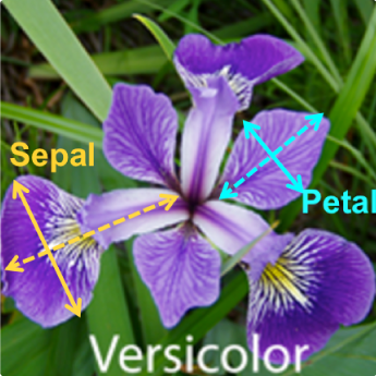
Iris flower has 3 species named “Setosa”, “Virginica” and “Versicolor”. These are classified based on length and width of sepals and petals the flower has.
Petals are modified leaves that surround the reproductive parts of flowers. They are often brightly colored or unusually shaped to attract pollinators. Where Sepals are a little support structure underneath the petal which typically function as protection for the flower in bud. Below diagram shall give fair idea about petals, sepals and their length-width.
So there are four features our dataset has:
-
Length of Sepal in centimeters
-
Width of Sepal in centimeters
-
Length of Petal incentimeters
-
Width of Petal incentimeters
Based on the combination of these four features, Iris flower is classified into different
3 species. For example,
| Flower# | Sepal Length | Sepal Width | Petal Length | Petal Width | Species |
|---|---|---|---|---|---|
| 1 | 5.1 | 3.5 | 1.4 | 0.2 | Iris setosa |
| 2 | 4.9 | 3.0 | 1.4 | 0.2 | Iris setosa |
| 3 | 7.0 | 3.2 | 4.7 | 1.4 | Iris versicolor |
| 4 | 6.4 | 3.2 | 4.5 | 1.5 | Iris versicolor |
| 5 | 6.7 | 3.3 | 5.7 | 2.5 | Iris virginica |
| 6 | 6.7 | 3.0 | 5.2 | 2.3 | Iris virginica |
We do have 150 records in this multivariate dataset and can be downloaded from here. So let’s dive in to classify these Iris higher dimensional dataset and further predict Iris species for any new data feed to our prediction system.
Pre-requisites for hands-on
In order to try out given example source code, you need python (either 2.7 or 3.x) setup on your system. Optionally you can use some IDE like pycharm or canopy for python code development.
Further below few python packages are required to be installed which helps doing statistics and machine learning. All of these packages may not be required to try out code given here but it is recommended to have them to be all set for learning and statistical code development environment.
Use “pip (or pip3) install {package_name}” command to deploy these python packages. If any additional dependencies prompted during installation then setup them as well.
To start with setup python-dev environment, for instance, on Ubuntu, you need to set it up using “apt-get install python-dev”.
Python packages to be deployed are:
| Package Name | Usage |
|---|---|
| scikitlearn | Opensource having simple and efficient tools for data mining and data analysis. It leverages below numpy, scipy internally. |
| numpy | Fundamental package for scientific computing using python. Sophisticates managing N-dimensional array object. |
| scipy | open-source software for mathematics, science, and engineering |
| matplotlib | For comprehensive 2D plotting and data visualizing |
| pandas | Open source, BSD-licensed library providing high-performance, easy-to-use data structures and data analysis tools for the Python programming language. Helps reading data from different file formats into in-memory dataframes. |
SVM (Support Vector Machine) – For Multivariate Dataset Classification
Ok, with Python development environment all set, let’s do Iris dataset classification using Support Vector Machines (SVM), which is a very advanced technique of clustering or classifying higher dimensional data.
“Support Vector Machines” (SVM) is a supervised learning technique as it gets trained using sample dataset. SVM is complex under the hood while figuring out higher dimensional support vectors or referred as hyperplanes across which to divide the data forming different clusters.
SVM provides user to choose different kernel functions (or clustering/classification algorithms) to get better results for specific dataset nature. There are various kernel options available like “linear” (which is linear regression technique), “poly” (for nonlinear or polynomial regression), “rbf” etc. For things like polynomial SVC (Support Vector Classifier) right degree polynomial is required to be used to tune for better results.
Though SVM is complex under the hood, the scikit-learn package makes it very easy to use without having to actually deep dive into it.
So here is python code snippet to form a linear kernel model for our Iris dataset using SVC technique.
Let’s open a new Python code file named svm_for_multivariate_data.py to code. As mentioned earlier, you can use any Python editor like pycharm, Canopy if you like or use any text editor to write below given code snippets.
Note: You can run the program from command line using “python svm_for_multivariate_data.py”
“””
This code demonstrates SVM(Support Vector Machine) for classification of multi-dimensional Dataset.
Please refer here a sample dataset of Iris flowers having multiple dimensions i.e.
petal-length, petal-width, sepal-length, sepal-width.
You can do “wget https://archive.ics.uci.edu/ml/machine-learning-databases/iris/iris.data” to save this dataset locally. Or optionally you can also refer this URL directly while loading dataframe.
“””
import pandas as pd
from sklearn import model_selection
from sklearn import svm
# Read dataset into pandas dataframe
df = pd.read_csv(‘/your_path_for_input_dataset/iris.data’,names=[‘sepal-len’, ‘sepal-width’, ‘petal-len’, ‘petal-width’,’target’])
iris_features = [‘sepal-len’, ‘sepal-width’, ‘petal-len’, ‘petal-width’]
# Extract features
X = df.loc[:, iris_features].values
# Extract target i.e. iris species
Y = df.loc[:, [‘target’]].values
# Now using scikit-learn model_selection module, split the iris data into train/test data sets
# keeping 40% reserved for testing purpose and 60% data will be used to train and form model.
X_train, X_test, Y_train, Y_test = model_selection.train_test_split (X, Y, test_size=0.4, random_state=0)
# Build an SVC (Support Vector Classification) model using linear regression
clf_ob = svm.SVC(kernel=’linear’, C=1).fit(X_train, Y_train)
So with hardly few lines of code, SVC model for Iris dataset got trained and ready to use predicting Iris species for new dimensions.
But how do we know our model built is robust or accurate enough. We can measure this model performance using the reserved test data.
print(clf_ob.score(X_test, Y_test))
This shall print score result around 0.966666666667 which is quite good (x->1 is better where x->0 is worst) but as you can see it is based on only some random dataset used for training purpose and rest for testing. Such model might not be actually robust due to different reasons like,
-
May show high score due to overfitting of train and test datasets, as probably the dataset are similar or they have similar outliers.
-
May not show good score due to small datasets or train,test datasets are not good enough.
-
As trained and tested only once using sample datasets, model may not be well aware of bias and variance in data.
So, how to validate the model robustness? Use K-Fold Cross Validation technique
Basic concept behind K-Fold cross validation is train-and-test is tried multiple times. So data is not split into just one training set and testing set but into multiple randomly assigned segments, K-segments. At high level it works like below:
-
Dataset is divided into K random segments
-
One of the segments is reserved for testing or validation purpose
-
For each K-1 segments it does training and measures score against the test dataset
-
Average of the K-1 scores is calculated to present more robust score of the classification model.
Here is code snippet for K-Fold cross validation against the SVC model with linear kernel constructed for the Iris dataset.
# Further, let’s now validate robustness of above model using K-Fold Cross validation technique
# We give cross_val_score a model, the entire iris data set and its real values, and the number of folds:
scores_res = model_selection.cross_val_score(clf_ob, X, Y, cv=5)
# Print the accuracy of each fold (i.e. 5 as above we asked cv 5)
print(scores_res)
# And the mean accuracy of all 5 folds.
print(scores_res.mean())
Here cv=5 stands for use 5 folds or runs using different training datasets. This code snippet gives 5 folds score something like below and mean score around 0.98 which denotes the model is indeed working pretty good. Notice that it is greater than score 0.966666666667 discovered earlier using one pass.
[0.96666667, 1., 0.96666667, 0.96666667, 1.]
0.98
Predict category of new data
This model now can be used to predict new Iris flowers species using their given sepal length-width and petal length-width. Let’s use below dataset. Their species are given for reference. The model shall predict the species correctly.
| Flower# | Sepal Length | Sepal Width | Petal Length | Petal Width | Species |
|---|---|---|---|---|---|
| 1 | 4.9876 | 3.348 | 1.8488 | 0.2 | Iris setosa |
| 2 | 5.3654 | 2.0853 | 3.4675 | 1.1222 | Iris versicolor |
| 3 | 5.890 | 3.33 | 5.134 | 1.6 | Iris virginica |
Append below python code lines and run the program.
in_data_for_prediction = [[4.9876, 3.348, 1.8488, 0.2], [5.3654, 2.0853, 3.4675, 1.1222], [5.890, 3.33, 5.134, 1.6]]
p_res = clf_ob.predict(in_data_for_prediction)
print(‘Given first iris is of type:’, p_res[0])
print(‘Given second iris is of type:’, p_res[1])
print(‘Given third iris is of type:’, p_res[2])
Indeed, it gives expected output:
Given first iris is of type: Iris-setosa
Given second iris is of type: Iris-versicolor
Given third iris is of type: Iris-virginica
Dimensionality Reduction concept and associated technique
As indicated earlier, as dataset has higher and higher dimensions it becomes difficult to visualize dataset classification. We cant’t imagine hyperplanes more than 3 axes. Not only just visualization but if dataset to be classified has a lot of features and it is big in size as well then often it impacts management as well as analysis speed.
For this reason, dimensionality reduction techniques helps to figure out way to reduce higher dimensional information into lower dimensional information. Not only can that make it easier to look at, and classify things, but it can also be useful for things like compressing data.
While compressing data and reducing dimensions it also helps preserving maximum amount of variance from original dataset.
Usually when Dimensionality Reduction topic is talked over, PCA (Principal Component Analysis) technique is reffered.
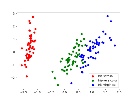
Let’s see how can we use PCA technique to reduce Iris 4-Dimensional dataset into 2- Dimensional format, by still keeping variance as in original dataset, and simplifying dataset visualization.
Below code snippet transforms 4-D into 2-D dataset; prints preserved variance of original dataset which comes around 0.977631775025 which is quite good (x->1 is good).
“””
Dimensionality Reduction using PCA (Principal Component Analysis) Here n_components = 2 means, transform into a 2-Dimensional dataset.
“””
pca = PCA(n_components=2, whiten=True).fit(X)
X_pca = pca.transform(X)
print(‘explained variance ratio:’, pca.explained_variance_ratio_)
print(‘Preserved Variance:’, sum(pca.explained_variance_ratio_))
# Print scatter plot to view classification of the simplified dataset
colors = cycle(‘rgb’)
target_names = [‘Iris-setosa’, ‘Iris-versicolor’, ‘Iris-virginica’]
pl.figure()
target_list = array(Y).flatten()
for t_name, c in zip(target_names, colors):
pl.scatter(X_pca[target_list == t_name, 0], X_pca[target_list ==t_name, 1], c=c, label=t_name)
pl.legend()
pl.show()
Transformed 2-D data looks something like below for a couple of records in our original 4-D dataset.
Original Dataset Records:
| Flower# | Sepal Length | Sepal Width | Petal Length | Petal Width | Species |
|---|---|---|---|---|---|
| 0 | 5.1 | 3.5 | 1.4 | 0.2 | Iris setosa |
| 70 | 5.9 | 3.2 | 4.8 | 1.8 | Iris versicolor |
| 120 | 6.9 | 3.2 | 5.7 | 2.3 | Iris virginica |
Transformed Dataset Records:
| Flower# | X axis | Y axis | Species |
|---|---|---|---|
| 0 | -1.3059028 | 0.66358991 | Iris-setosa |
| 70 | 0.5430661 | -0.17110324 | Iris-versicolor |
| 120 | 1.18133597 | 0.76553312 | Iris-virginica |
Using matplotlib library, a scatter plot is printed for this transformed data which looks something like below. Run the program to view preserved variance and scatter plot.
Summary
Well, this covers gist about handling multivariate dataset, making classifications, doing predictions and also simplifying into lower dimensions for data compression and better visualization purpose. The scope & complexity keeps growing when dataset size to be handled is huge. In a way, it becomes Big Data problem statement.
Stay tuned for further blog on Machine Learning for Big Data having higher dimensions. Thank you !!!
© 2018 Isana Systems